Principal Components Analysis in R: College Sports

Last fall, I took a multivariate statistics course at the University of Kansas as part of the Applied Statistics, Analytics, and Data Science graduate program. One of the topics covered in the course was principal components analysis (PCA). PCA is commonly used when 1. there are a large number of numerical variables in a data set, and 2. the variables are strongly correlated with each other. After conducting a PCA, the correlated variables can be replaced by a smaller number of uncorrelated variables, known as the principal components. Each principal component is a linear combination of the original variables that represents most of the information, or variability, found in the original variables.

For this demonstration, I am using a data set on college sports provided by the TidyTuesday data project. This data set contains several variables on athletic participation, staffing, and finances by college, sport, and team gender. Since the numeric variables are on different scales, e.g., rev_women is in dollars, while partic_women is counts of women, they will inevitably have different variances. To account for the different variances, we will perform a PCA on the correlation matrix which uses the standardized data, as opposed to the covariance matrix which uses the non-standardized data.

Let’s create a correlation heatmap using ggplot2 to visualize the correlations between the numerical variables. Figure 1 displays the Pearson correlation coefficient between all numerical variables in the college sports data set in a heatmap.

tuesdata <-
  tidytuesdayR::tt_load('2022-03-29')

sports <- tuesdata$sports %>%
  select_if(is.numeric) %>%
  select(-c(contains("code"), unitid, sector_cd))

sports_corr <- round(cor(sports, use = "complete.obs"), 2) %>%
  reshape2::melt()

sports_corr %>%
  ggplot(aes(Var1, Var2, fill = value)) +
  geom_tile() +
  geom_text(aes(label = value), color = "white", size = 2.2) +
  coord_fixed() +
  scale_fill_gradient2(low = "#E69F00",
                       mid = "#56B4E9",
                       high = "#009E73") +
  theme(axis.text.x = element_text(angle = 45,
                                   hjust = 1)) +
  labs(x = "", y = "",
       fill = "corr")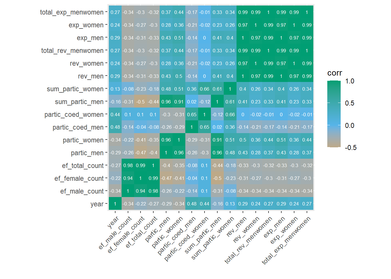

Figure 1: College sports data correlation heatmap

From the heatmap, we can see strong linear correlations between several variables, such as: total number of female students (ef_female_count) and total number of male students (ef_male_count) (r = 0.94), number of women participants (partic_women) and number of male participants (partic_male) (r = 0.96), and revenue in USD for men (rev_men) and revenue in USD for women (rev_women) (r = 0.97). Pairs of variables with a correlation of nearly 1 are those that are used to calculate each other, for example, total_rev_menwomen is the sum of rev_men and rev_women. Let’s remove these redundant variables and proceed to the next step.

sports_data <- 
  sports %>%
  select(-contains("total"), -contains("sum"))

We can use the prcomp() function with the scale. argument set to TRUE to run our PCA on the normalized data. We can also use the na.omit() function to remove missing values. Due to the large amount of missing values in this data set, we are left with 16 complete observations.

The first four principal components account for 93.5% of the total variability in the original variables, in other words, we can explain most of the variability in the data using four principal components, rather than the original 13 variables.

sports_pc <- prcomp(na.omit(sports_data), scale. = TRUE)
summary(sports_pc)

## Importance of components:
##                           PC1    PC2    PC3     PC4     PC5    PC6     PC7
## Standard deviation     2.2227 1.5959 1.3281 1.01933 0.60966 0.5410 0.17617
## Proportion of Variance 0.4491 0.2315 0.1603 0.09446 0.03379 0.0266 0.00282
## Cumulative Proportion  0.4491 0.6806 0.8410 0.93544 0.96923 0.9958 0.99865
##                            PC8     PC9    PC10      PC11
## Standard deviation     0.11813 0.02903 0.00206 0.0007071
## Proportion of Variance 0.00127 0.00008 0.00000 0.0000000
## Cumulative Proportion  0.99992 1.00000 1.00000 1.0000000

As a reminder, the principal components are linear combinations of the original variables that aim to contain most of the information and variability present in the original variables. The prcomp() function also saves the weights given to each variable within each component in the rotation element of the prcomp() output. We can see that the largest positive weights in the first principal component are for the revenue and expenditure variables. In the second principal component, the largest negative weight is for year, followed by the coed participation variables. These weights are then used to calculate principal component scores.

sports_pc$rotation[, 1:4]

##                           PC1         PC2         PC3         PC4
## year               0.08046550 -0.52461564  0.09271418 -0.12001052
## ef_male_count     -0.24314197  0.13690902 -0.54595277  0.32460550
## ef_female_count   -0.25016590  0.02608413 -0.59768741  0.15966536
## partic_men         0.27528119  0.34598572  0.22519978  0.43011892
## partic_women       0.29553703  0.35072278  0.14609532  0.43437032
## partic_coed_men   -0.10270443 -0.44259190  0.24378571  0.42958896
## partic_coed_women -0.06919406 -0.46034026 -0.02641298  0.51493408
## rev_men            0.42553268 -0.10892997 -0.19470486  0.05995430
## rev_women          0.40685332 -0.12511926 -0.25329927 -0.11009306
## exp_men            0.42558205 -0.10843060 -0.19470472  0.05983943
## exp_women          0.40698729 -0.12475127 -0.25286576 -0.10980126

The principal component scores are saved in the x element of the prcomp() output. High scores on the first principal component indicate that the revenue and expenditures of that college sport are high. High scores on the second principal component indicate that the year is further in the past and that coed participation is low.

sports_pc$x[, 1:4]

##              PC1        PC2         PC3         PC4
##  [1,]  0.6299691  2.7610736  0.78941093  0.86377070
##  [2,]  0.8820529  2.2771150  0.78977817  0.71723087
##  [3,] -3.1135609  1.4213659 -2.75558053  0.40061779
##  [4,]  0.8959289  1.7376713  0.89874487  0.42684134
##  [5,]  1.9306728 -0.2859732 -0.70887921 -1.25939102
##  [6,] -1.7094386 -0.1181410  0.89276872 -0.96397899
##  [7,] -2.7431012  0.8567710 -2.36512376  0.09115136
##  [8,]  0.9809652  1.0637934  0.78367389  0.03255717
##  [9,] -1.5544257 -0.6958294  1.23024817 -0.92098308
## [10,]  6.2495058 -0.8904998 -1.67719480  0.15392365
## [11,] -1.2379055 -3.1809537  0.45968955  2.58756770
## [12,] -1.5550160 -0.6634227  0.51784857 -1.05954324
## [13,] -0.2122136 -0.7192470  0.78114954 -1.46269840
## [14,]  1.0836685 -1.3051982 -1.23241388 -0.43238132
## [15,]  0.2436582 -0.1845523  1.53686975  0.63695381
## [16,] -0.7707599 -2.0739730  0.05901003  0.18836166

If our goal is to reduce the number of predictors in the data, we can use the first four columns of principal component scores as our transformed predictors. These four transformed predictors are now able to explain 93.5% of variability that was present in the original 13 variables. However, it is important to keep in mind that PCA only focuses on the linear relationships between the original variables, and any information in nonlinear relationships is not captured.